Symmetrized Covariant Derivatives
Introduction
A
symmetrized derivative covariant derivative is symmetrization of a number of covariant derivatives:
The main advantage of symmetrized derivatives is that they have a greater degree of symmetry than non-symmetrized (or ordinary) derivatives. For instance, it is obvious that the following is zero:
However, when we write out the symmetrized derivative, it is not immediately clear that the expression is zero:
Of course, when we write
![F^([ab]) ∇_a∇_b F^([ab]) ∇_a∇_b](Files/SymmetrizedDerivatives/Image_4.gif)
as a commutator, we recover zero. But the point is that eliminating commutators is something the xTensor canonicalizer does not do. So it is often necessary to explicitly symmetrize covariant derivatives in order to fully canonicalize an expression.
Implementation
Functions for symmetrizing and de-symmetrizing covariant derivatives.
Symmetrized covariant derivatives are implement in xTras as follows. Whenever a covariant derivative
CD is defined to be
symmetrizable,
CD[-a,-b] will mean

(and likewise for more indices). A covariant derivative can be defined to symmetrizable by giving the option
SymCovDQ -> True to
DefCovD or
DefMetric:
Now define a metric and covariant derivative. We need to specify SymCovDQ in order to make the covariant derivative symmetrizable.
Derivatives with more than one index are now interpreted as symmerized derivatives:
| Out[20]= |  |
| Out[21]= |  |
We can expand the symmetrized derivative with a call to
ExpandSymCovDs:
| Out[22]= |  |
Single derivatives can be symmetrized with
SymmetrizeCovDs:
| Out[23]= |  |
| Out[24]= |  |
Symmetrized derivatives are automatically Leibnitz:
| Out[25]= |  |
Integrating by parts can be done with
VarD:
| Out[29]= |  |
Notice that two symmetrized derivatives acting on each other are not automatically symmetrized further. We need to call
SymmetrizeCovDs again to do so explicitly:
| Out[31]= |  |
However, when we set
$AutoSymmetrizeCovDs to True, all derivatives that are not fully symmetrized will automatically get symmetrized:
| Out[32]= |  |
| Out[34]= |  |
By setting
$AutoSymmetrizeCovDs to False we return to the default behaviour:
| Out[35]= |  |
| Out[36]= |  |
Because symmetrizing derivatives is a an operation the grows exponentially in complexity (see the section on performance below), the function
SymmetrizeCovDs stores its results in the variable
$SymCovDCache. The cache can be cleared with
ClearSymCovDCache:
| Out[44]= |  |
By default, symmetrizations are cached:
| Out[45]= |  |
Subsequent symmetrizations are then faster:
| Out[46]= |  |
But the first symmetrization was slower compared to when no cache is used:
| Out[47]= |  |
This is because
SymmetrizeCovDs spents some time on store the results in the cache. If you plan on symmetrizing a lot of derivatives, using the cache is faster in the long run.
Performance
The implementation of symmetrizing derivatives is exponentially complex in the number of derivatives.
SymmetrizeCovDs has an optimized algorithm in the case when there is no torsion. Whenever there is torsion, a slower algorithm is used.
Properties of symmetrized derivatives
Below we list some useful formulas and properties of symmetrized derivatives.
Symmetrizing
Because it is always possible to commute adjacent covariant derivatives by introducing curvature, a symmetrized covariant derivative can in general be expressed as
By induction, we can deduce that a single ordinary derivative can be eaten by a symmetrized derivative as follows:
where the general commutator operator

is given by
Although it is not explicitly indicated after the last equal sign because it would clutter notation, all

indices above are symmetrized over.
This expression for the operator

is not completely closed; it contains terms of the form
for which it is quite hard to find a closed formula relating it to

.
However, whenever there is no torsion, the operator

can be expressed as
where the commutator in the first term does not act on the indices of

, but only on the expression on which the operator

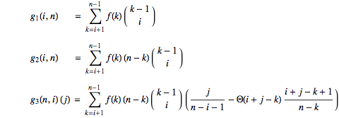
acts. Furthermore, the numeric functions

are given by
where

is the
UnitStep function. Note that

with fixed

and

gets fed into the next iteration of

as its

).
A similar closed form for

with torsion should also exist.
Other properties
Distributivity is inherited from the ordinary derivative:
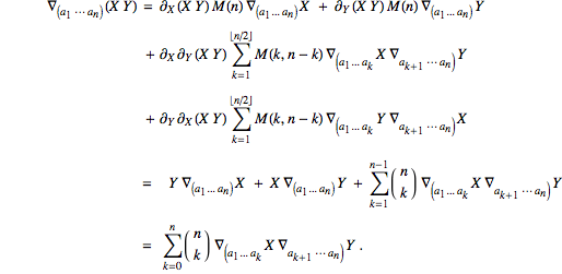
If the ordinary derivative is Leibnitz, we have the following generalization of the Leibnitz rule:
Counting the number of terms on boths sides provides a consistency check on this formula; the left-hand-side has

terms, the same as the right-hand-side, namely

.
Integrating by parts also carries over nicely:
Lastly, the action of a Leibnitz symmetrized derivative on a generic function

with arguments

can be written as the following generalized chain rule:
This a generalization of Faà di Bruno's formula. Here

, and the contracted

indices are summed over. Furthermore,

denotes the set of partitions of

into

integers

(to be precise,

is the result of
IntegerPartitions[n, {i}]). And

is the weighted multinomial
The generalized Leibnitz rule above is actually a limiting case of the generalized chain rule, as we can see by setting

:
Similarly, the distributivity property can also be derived from the generalized chain rule by setting

.
![F^([ab]) ∇_a∇_b F^([ab]) ∇_a∇_b](Files/SymmetrizedDerivatives/Image_4.gif) as a commutator, we recover zero. But the point is that eliminating commutators is something the xTensor canonicalizer does not do. So it is often necessary to explicitly symmetrize covariant derivatives in order to fully canonicalize an expression.
as a commutator, we recover zero. But the point is that eliminating commutators is something the xTensor canonicalizer does not do. So it is often necessary to explicitly symmetrize covariant derivatives in order to fully canonicalize an expression. (and likewise for more indices). A covariant derivative can be defined to symmetrizable by giving the option SymCovDQ -> True to DefCovD or DefMetric:

 indices above are symmetrized over.
 is not completely closed; it contains terms of the form
 .
. can be expressed as
 , but only on the expression on which the operator
  acts. Furthermore, the numeric functions
  are given by
 is the UnitStep function. Note that
  with fixed
  and
and  gets fed into the next iteration of
  as its
  ).
). with torsion should also exist.
 terms, the same as the right-hand-side, namely
  .
.  with arguments
  can be written as the following generalized chain rule:
 , and the contracted
  indices are summed over. Furthermore,
  denotes the set of partitions of
  into
into  integers
  (to be precise,
  is the result of IntegerPartitions[n, {i}]). And
  is the weighted multinomial
![∇_((ab))T^c= 1/2(∇_a∇_b+∇_b∇_a)T^c = 1/2(∇_a∇_b+∇_a∇_b+∇_b∇_a-∇_a∇_b)T^c = (∇_a∇_b+1/2[∇_b,∇_a])T^c = ∇_a∇_b T^c+1/2R_(abd)^cT^d+1/2T_(ab)^d∇_dT^c . ∇_((ab))T^c= 1/2(∇_a∇_b+∇_b∇_a)T^c = 1/2(∇_a∇_b+∇_a∇_b+∇_b∇_a-∇_a∇_b)T^c = (∇_a∇_b+1/2[∇_b,∇_a])T^c = ∇_a∇_b T^c+1/2R_(abd)^cT^d+1/2T_(ab)^d∇_dT^c .](Files/SymmetrizedDerivatives/Image_9.gif)
![D[f(i)]_(a_1...a_n, b) = ∑_(i=0)^(n-1) g_1(i,n) (∇_(a_1... a_i)[∇_b,∇_(a_(i+1))])∇_(a_(i+2)... a_n) + ∑_(i=0)^(n-2)g_2(i,n)(∇_(a_1... a_i)R_(ba_(i+1)a_(i+2))^c)∇_(a_(i+3)... a_nc) -∑_(i=0)^(n-3)(∇_(a_1... a_i)R_(ba_(i+1)a_(i+2))^c)D[g_3(n,i)(j)]_(a_(i+3)...a_n, c) D[f(i)]_(a_1...a_n, b) = ∑_(i=0)^(n-1) g_1(i,n) (∇_(a_1... a_i)[∇_b,∇_(a_(i+1))])∇_(a_(i+2)... a_n) + ∑_(i=0)^(n-2)g_2(i,n)(∇_(a_1... a_i)R_(ba_(i+1)a_(i+2))^c)∇_(a_(i+3)... a_nc) -∑_(i=0)^(n-3)(∇_(a_1... a_i)R_(ba_(i+1)a_(i+2))^c)D[g_3(n,i)(j)]_(a_(i+3)...a_n, c)](Files/SymmetrizedDerivatives/Image_19.gif)


