3. Canonical invariants
RInv Non-dual invariant
DualRInv Dual invariant
RInvs List of all non-dual invariants after a given step
DualRInvs List of all dual invariants after a given step
MaxIndex Maximum value of the index for the list of non-dual invariant after a given step
MaxDualIndex Maximum value of the index for the list of dual invariants after a given step
RInvRules List of all independent invariants for a given step and case
RemoveRInvRules Remove rules for invariants of a given step and case
Canonical invariants
For a given case {![]() , ...,
, ..., ![]() }, there will be N! different monomials, where N = 4n +
}, there will be N! different monomials, where N = 4n +![]()
![]() , as we saw in the previous section. It is obviously impossible to store them all.
, as we saw in the previous section. It is obviously impossible to store them all.
Consider, for example, the numbers of possible permutations taking into acount only algebraic invariants, for wich the number of indices is N = 4n:
In[54]:=
![]()
Out[54]//TableForm=
| degree | number of monomials | |
| 1 | 24 | 24. |
| 2 | 40320 | 40320. |
| 3 | 479001600 | 4.79002*10^^8 |
| 4 | 20922789888000 | 2.09228*10^^13 |
| 5 | 2432902008176640000 | 2.4329*10^^18 |
| 6 | 620448401733239439360000 | 6.20448*10^^23 |
| 7 | 304888344611713860501504000000 | 3.04888*10^^29 |
We can, however, store the corresponding canonical invariants with respect to permutation symmetries. The numbers of canonical invariants for each case are stored in the functions MaxIndex and MaxDualIndex,
In[55]:=
![]()
Out[55]=
![]()
For example, the values up to order 10 are
In[56]:=
![]()
Out[56]//MatrixForm=

In[57]:=
![]()
Out[57]=
![]()
In[58]:=
![]()
Out[58]=
![]()
Within each case, the canonical invariants are labeled (Dual)RInv[metric][case, index], where index is an integer ranging from 1 to Max(Dual)Index[case]. Non dual invariants are output as ![]() , where case, for brevity and clarity, is not the list {
, where case, for brevity and clarity, is not the list {![]() , ...,
, ..., ![]() }, but simply the concatenation of its elements
}, but simply the concatenation of its elements ![]()
![]() ...
...![]() . Notice that there is no confusion because the
. Notice that there is no confusion because the ![]() are always single digit integers, except for the case {10}, but even then there is no problem, because we always write the
are always single digit integers, except for the case {10}, but even then there is no problem, because we always write the ![]() in increasing order. Dual invariants are represented by
in increasing order. Dual invariants are represented by ![]() .
.
Examples:
In[59]:=
![]()
Out[59]=
![]()
In[60]:=
![]()
Out[60]=
![]()
As we apply more symmetries, the lists of independent (Dual)RInvs get smaller. We can produce the independent invariant at each simplification step with the command (Dual)RInvs[metric][step, case]. The first step produces a list of length MaxIndex[case]
In[61]:=
![]()
Out[61]=

In[62]:=
![]()
Out[62]=

After applying the cyclic identity we get
In[63]:=
![]()
![]()
Out[63]=

After the Bianchi identity
In[64]:=
![]()
![]()
Out[64]=
![]()
After reordering derivatives
In[65]:=
![]()
![]()
Out[65]=
![]()
After the dimensionally dependent identities
In[66]:=
![]()
![]()
Out[66]=
![]()
In this case there are no signature dependent relations (= relations arising from products of dual invariants)
In[67]:=
![]()
![]()
Out[67]=
![]()
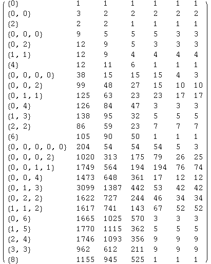
The following table reproduces the one in the paper listing the numbers of invariants after each step for all cases up to order 10
In[68]:=
In[69]:=
![]()
Out[69]//MatrixForm=

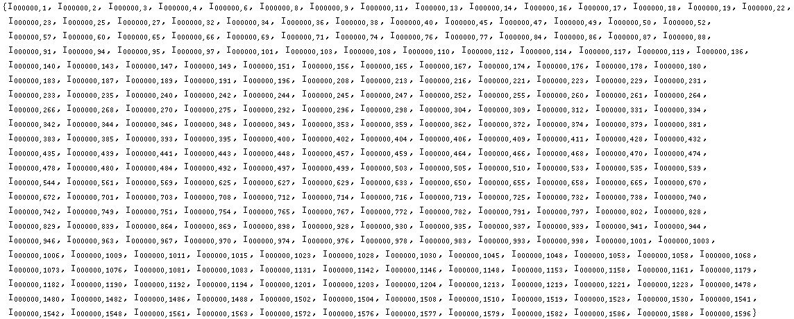
The simplified notation RInvs[metric][step, n] is automatically translated into RInvs[metric][step, {0, ![]() , 0}], for backwards compatibility with Invar 1. For instance, these are all the algebraic invariants after step 3 with degree 6 (case {0,0,0,0,0,0}):
, 0}], for backwards compatibility with Invar 1. For instance, these are all the algebraic invariants after step 3 with degree 6 (case {0,0,0,0,0,0}):
In[70]:=
![]()
![]()
![]()
Out[70]=

Similar shorthands are available for other commands, such as MaxIndex or RInv
In[71]:=
![]()
Out[71]=
![]()
In[72]:=
![]()
Out[72]=
![]()
In[73]:=
![]()
![]()
Out[73]=

If we restrict ourselves to algebraic invariants we can give a basis of only 25 invariants (notice that there is no step 6 for dual invariants)
In[74]:=
![]()
![]()
![]()
![]()
![]()
![]()
![]()
![]()
![]()
![]()
![]()
![]()
![]()
![]()
![]()
![]()
![]()
![]()
![]()
![]()
Out[74]=
![]()
In[75]:=
![]()
![]()
![]()
![]()
![]()
![]()
Out[75]//TableForm=
| Created by Mathematica (May 16, 2008) |